Ward 2022: CO₂ breakthrough curves
In Ward & Pini’s study, they analyzed dynamic breakthrough experiments for a CO₂/Air mixture with activated carbon by fitting a 1D transient breakthrough model to experimental data. In this tutorial we will explain how the results of this paper are replicated using Skarstrom.
1. Load the simulation data
In the menu bar, under "Examples", hover over "Ward_2022" and select "Ward_2022_Q=100[ccm].json".
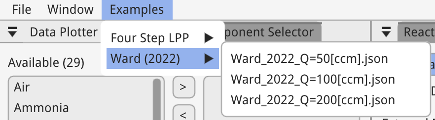
This will load all of the simulation data for the experiment with an inlet volumetric flow rate of 100 ccm. In the paper different internal heat transfer coefficients were used for each experiment, hence we have three simulation files.
2. Components
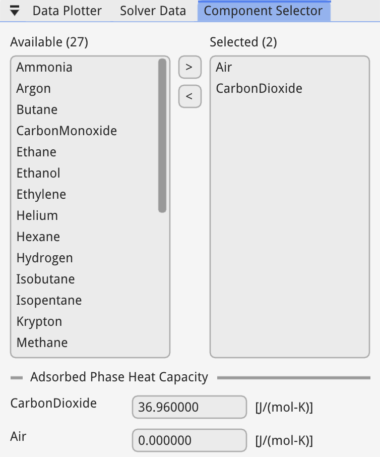
In the "Component Selector" window, make sure CO₂ and Air are selected.
The thermophysical properties of each component are calculated using CoolProp.
Ward models the adsorbed phase heat capacity and it can be specified in this window.
3. Reactor Properties
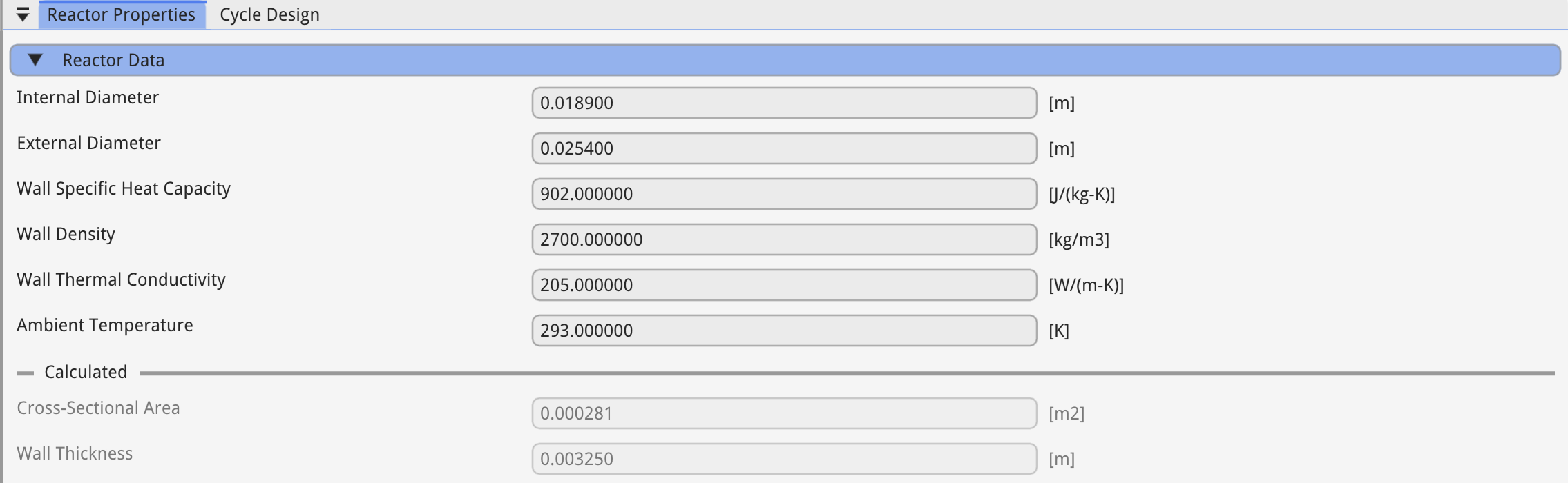
In the reactor properties window, you can specify the internal and external diameter along with the wall properties and ambient temperature.
The wall is made from aluminium and so the wall properties reflect that.
Next, the internal and external heat transfer coefficient equations can be selected.
Ward uses a constant internal heat transfer coefficient and the Holman (2008) equation for external heat transfer coefficient with a external velocity of 0.5 m/s.
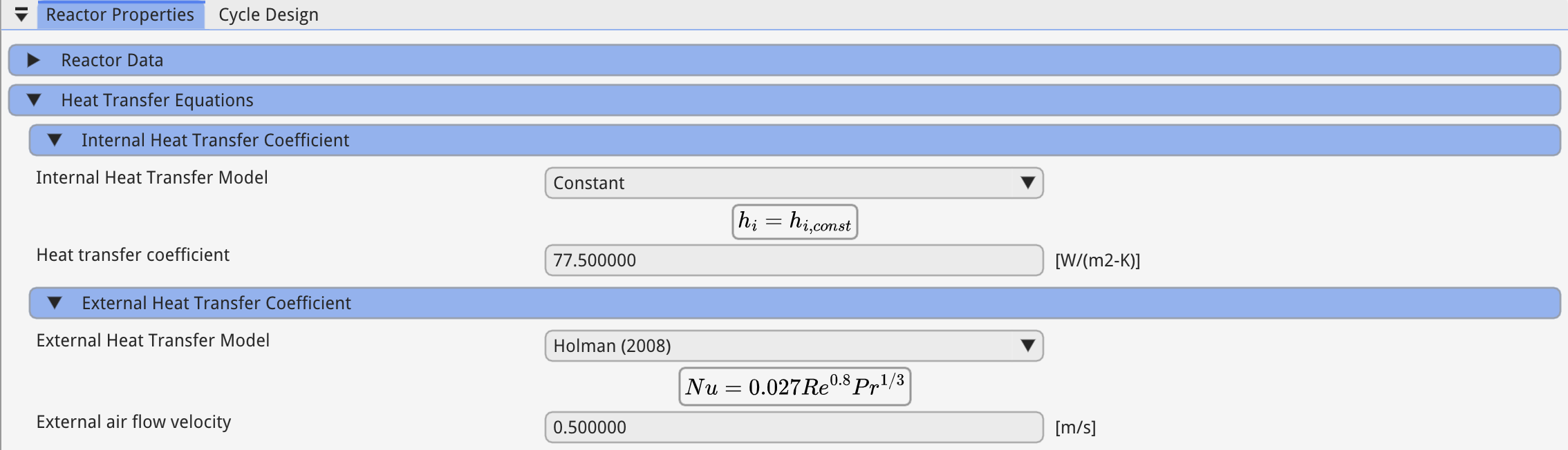
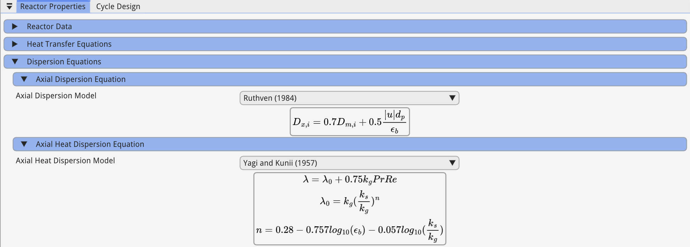
Now the equations used to calculate the dispersion coefficient are specified.
The mass dispersion equation is Ruthven (1984) and the axial thermal conductivity is Yagi and Kunii (1957).
4. Adsorbent Properties
Multi-layered beds can be created in Skarstrom, but for this simulation a single layer is required.
Select the "Activated Carbon" layer to open up the "Adsorbent Properties" window:
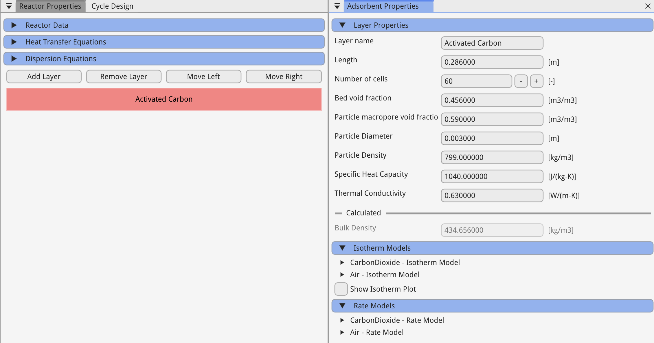
Here the length of the adsorbent domain, void fraction and other variables specific to the adsorbent layer are defined.
Each component requires an "Isotherm Model" which describes a components equilibrium adsorbed phase concentration,
and a "Rate Model" which describes the rate at which the adsorbed phase concentration changes with time, i.e. the mass transfer rate between the gas and solid.
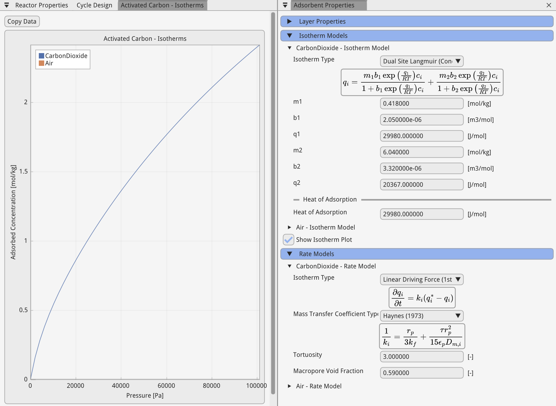
The isotherm used in Wards paper is the dual-site langmuir isotherm, concentration basis.
The rate model is the linear driving force, with the mass transfer coefficient calculated by the correlation suggested by Hayens (1973).
Isotherms can be visualised by selecting the "Show Isotherm Plot" checkbox.
5. Cycle Design
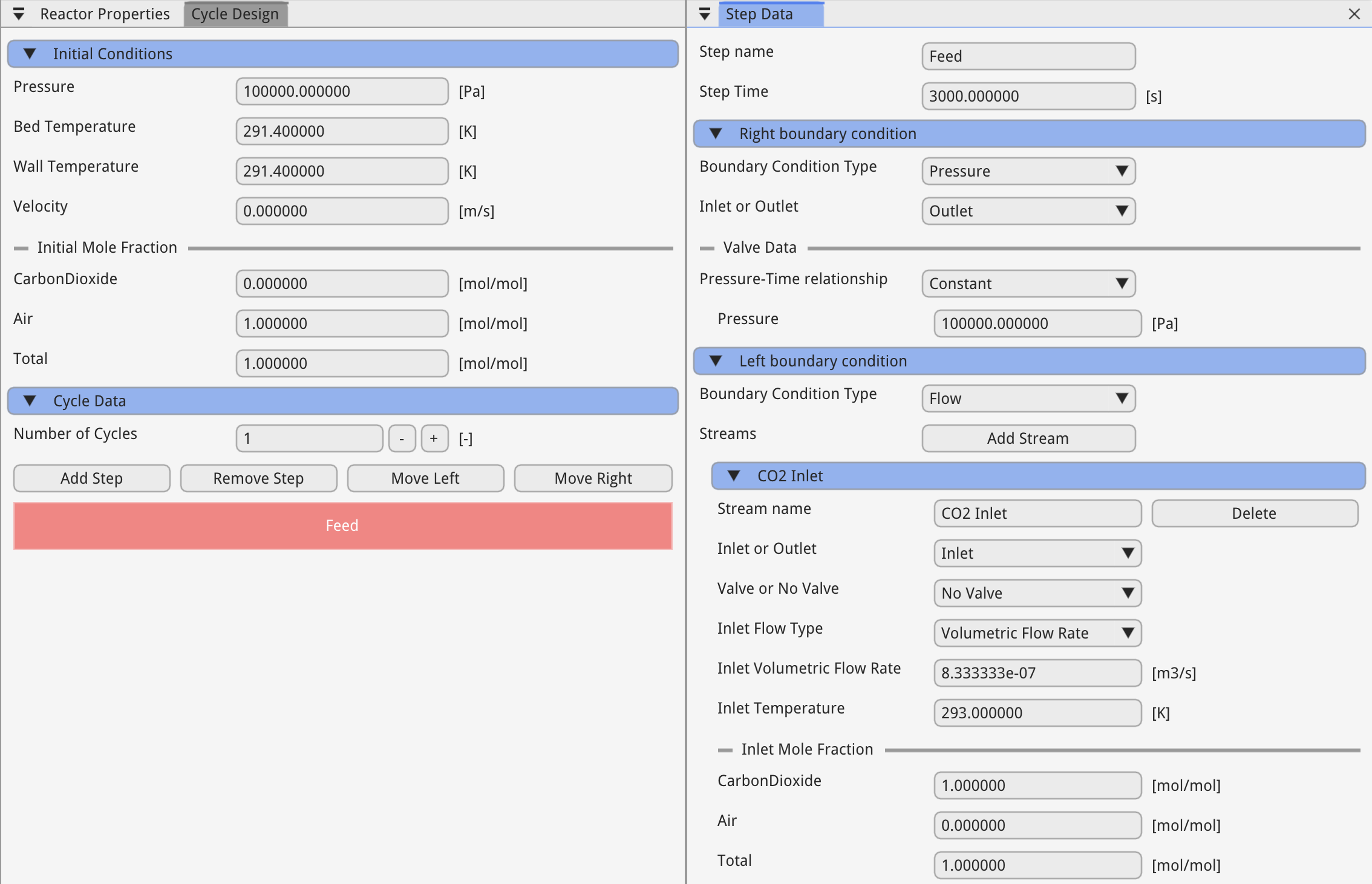
The cycle design for a breakthrough simulation is very straightforward, and requires a single step, with one cycle.
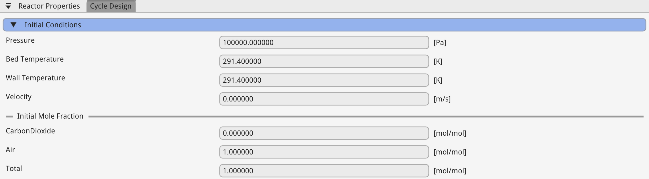
First you must specify the initial condition.
Ensure that the sum of mole fractions is equal to 1.
Next, select the "Feed" step to edit the step time and boundary conditions.
In Skarstrom, the right boundary condition is defined at and the left boundary condition defined at .
In a "flow-through" step, the inlet to the vessel specifies the volumetric flow rate, and the outlet boundary condition is constant pressure.
6. Solver
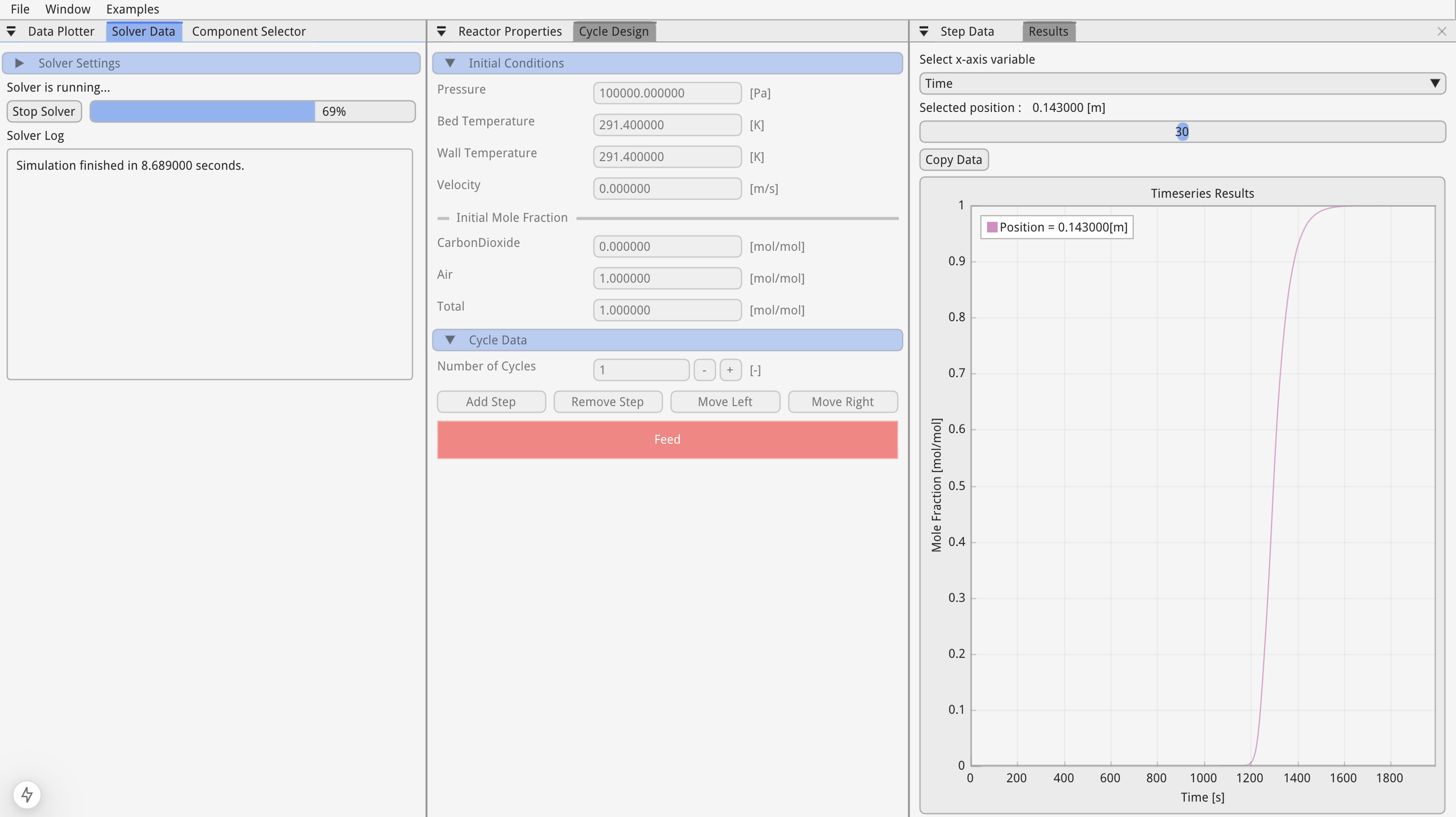
Now all of the model parameters are set up, we are ready to run the solver.
Select the "Solver Data" tab, and press "Run Solver".
This will disable the UI elements, but you can stil click on the "Data Plotter" window to visualise the data as the solver progresses.
7. Data Visualisation
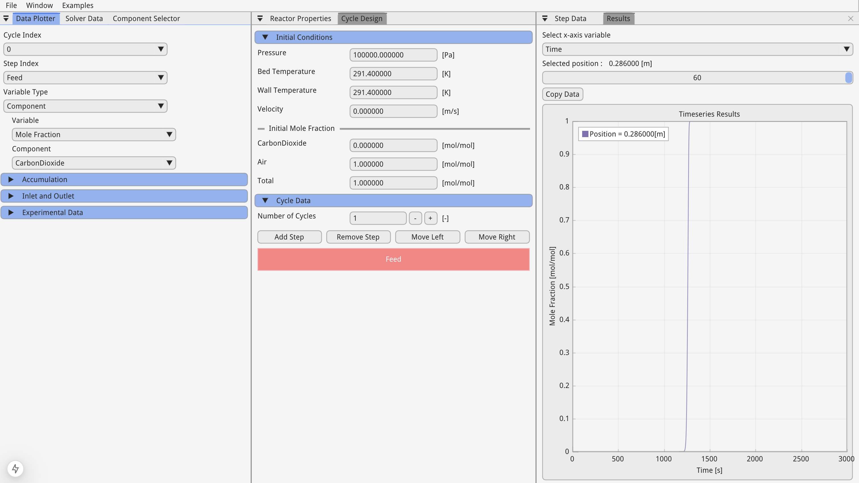
In the "Data Plotter" window variables are classified as "Bulk" or "Component".
"Bulk" variables refer to variables of the fluid such as pressure and temperature, whereas "Component" variables refer to those variables specific to a component within the fluid such as mole fraction.
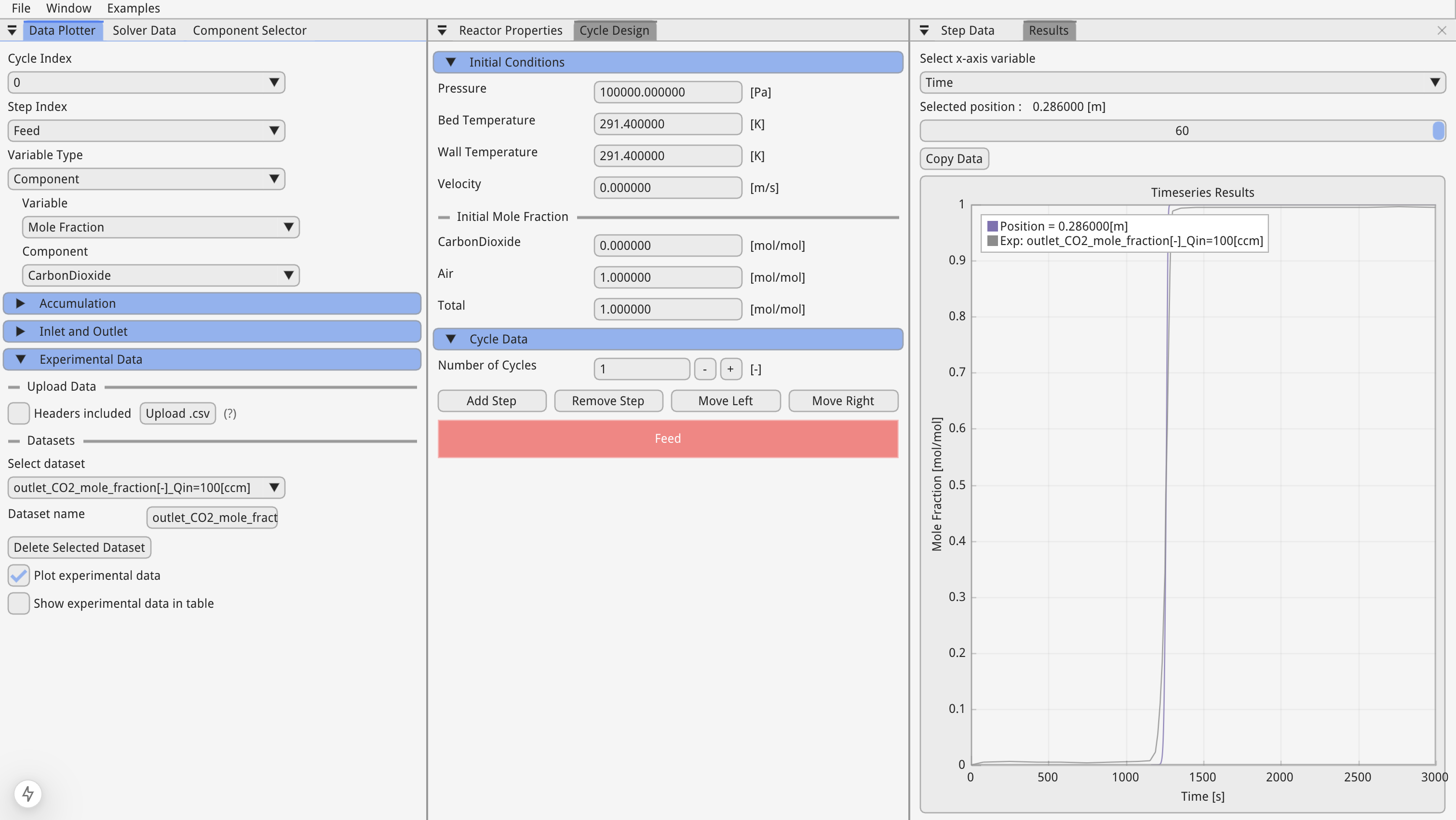
Selecting, "Component", "Mole Fraction" and "CarbonDioxide" we can move the position slider in the "Results" tab to the far right to plot the outlet CO₂ concentration with time.
8. Simulation Validation
To compare the simulation result with the data from Ward's paper, go to the "Data Plotter" windown and open the "Experimental Data" collapsing header.
Here you can upload data via .csv files and plot them against the simulation data.
We have pre-loaded the experimental date which can be selected in the drop down and plotted by selecting the "Plot experiment data" checkbox.